Python-Implementation-of-Hampel-Filter

Introduction

The Hampel filter is used to detect outliers in time series data. I wanted to use this filter to detect outliers in the sensor data collected from wearable sensors. However, the only implementation I could find [1] is implemented in Python using Pandas’s rolling() and apply() functions, which causes longer execution time as the input time series gets longer. Therefore, I reimplement this using NumPy for faster execution. The execution time of these two implementations, Pandas-based implementation [1] and my NumPy-based implementation, are compared at the end of this article.

My implementation is available here.

Hampel Filter

The algorithm of the Hampel Filter is as follows [2]:

For a given sample of data, $x_s$, the algorithm:

• Centers the window of odd length at the current sample.
• Computes the local median, $m_i$, and standard deviation, $\sigma_i$, over the current window of data.
• Compares the current sample with $n_\sigma \times \sigma_i$, where $n_\sigma$ is the threshold value. If $∣x_s−m_i∣>n_\sigma \times \sigma_i$, the filter identifies the current sample, $x_s$, as an outlier and replaces it with the median value, $m_i$.

So basically, the algorithm applies sliding window and computes the local median and standard deviation, and if the Median Absolute Deviation (MAD) of the sample ($∣x_s−m_i∣$) is bigger than the threshold, $n_\sigma \times \sigma_i$, the sample is treated as an outlier. You can control the sensitivity of the filter by changing $n_\sigma$. Its window size is also a configurable parameter.

Performance Comparison

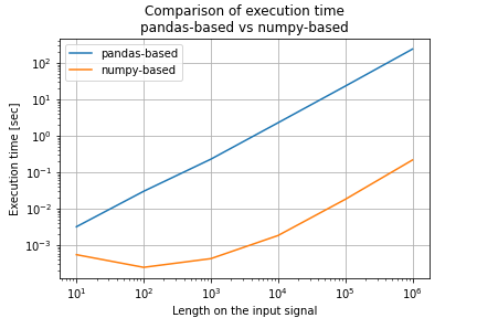
Figure 1. shows a comparison of execution times when the sample size is changed from 10 to 10^6. The horizontal axis is the length of the input signal (number of samples), and the vertical axis is the execution time. The execution time is proportionally increasing to the number of samples with the pandas-based implementation, whereas the execution time of the numpy-based implementation is not increasing until about n=10^3. After that, the execution time is linearly proportional to the number of samples for both, but the numpy-based implementation is about 10*3 times faster.

Figure 1. Comparison of execution times

Related Resources

• MichaelisTrofficus/hampel_filter (A Pandas-based implementation of the Hampel Filter)
• Filter outliers using Hampel identifier - Simulink
• Outliers in Process Modeling and Identification